Intro #

Imagine you’ve got this landscape-oriented photo but you want it to be square. In other words, you want to change its aspect ratio.

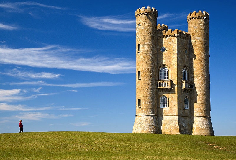
In this situation, you’ve got a few options: you either crop the image and lose maybe important or interesting parts of the image, or you accept the distortion because everything will be squeezed together. But what if there’s another option? That option listens to the name of content-aware scaling.

The idea #

Content-aware scaling takes into account – who would’ve thought! – the content when scaling an image. Instead of trying to cram all pixels into less (horizontal) space, why not omit the less interesting pixels in order to perform the resizing?

Finding the right energy #

The key is to find these “less interesting” pixels. The less interesting parts are definitely not the castle or the person standing on the left. If we take a look at the clear blue sky on the right side and remove some columns of pixels there, people would barely notice it.

The next question is, which columns exactly? And what other columns, apart from those on the right side, can we remove before we start to remove important parts? How do we calculate all of this?

Greyscale #

We start by turning the image into greyscale colours. In its most basic form, this comes down to summing up all three colour channels (red, green and blue) and dividing them by three to average them. More correct is to account for the relative luminance. The human eye is the most sensitive to green, then red and the least to blue. That gives the following formula¹:

$$ Y = 0.2126 * R + 0.7152 * G + 0.0722 * B $$

Convolve using an edge-detection kernel #

A kernel is a small matrix that is applied to every pixel (and its surrounding pixels) of an image with the goal to, for example, blur, sharpen, or, as I used it, highlight edges. The process of applying a kernel to every pixel of an image is called convolution and goes as follows:

• you loop over every value in the kernel;
• you multiply that value with the matching (surrounding) pixel value (e.g. the top-left kernel value gets multiplied by the pixel value of the pixel to the left and above the origin pixel);
• you sum up the result of all these multiplications;
• the final result is the new origin pixel’s value.

To give an additional example, the following kernel is like an identity matrix in the world of image processing:

$$ \begin{bmatrix} 0 & 0 & 0\\ 0 & 1 & 0\\ 0 & 0 & 0 \end{bmatrix} $$

An identity kernel is a “no-op” kernel: if you multiply all pixel values, the zeros cancel out the surrounding pixel values while the one in the middle keeps the origin pixel value, resulting in a net pixel value that is the same as before applying the kernel.

Sobel operator #

The Sobel operator is very useful for edge detection. It consists of two kernels, one for the horizontal gradient and one for the vertical gradient, indicating the change nearby pixels undergo. These kernels look like this (first horizontal, next vertical):

$$ \begin{bmatrix} 1 & 0 & -1\\ 2 & 0 & -2\\ 1 & 0 & -1 \end{bmatrix} $$

$$ \begin{bmatrix} 1 & 2 & 1\\ 0 & 0 & 0\\ -1 & -2 & -1 \end{bmatrix} $$

Combining both horizontal and vertical derivatives can be done by applying good ol’ Pythagoras’ theorem and will finally yield the new pixel’s value. If we apply these Sobel kernels to our image from above, we get the following result.

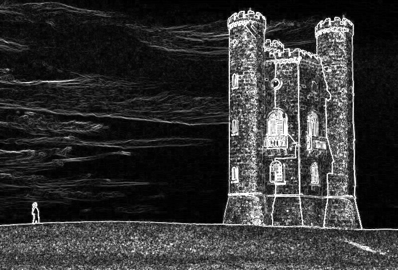
Notice how all edges are clearly visible – even the clouds! – and comprise the “more busy” or important parts of the image. These edges should be preserved and tried to not be selected first when choosing pixel columns (or rows) to remove. Finally, note our intuition was correct. The space to the right of the castle doesn’t contain a lot of change so this makes it an ideal location to remove some pixels from.

Compute the energy #

At this point, we’ve got a good view of the parts of the image that don’t contain a lot of visual changes. Next, we need to select a line or seam of pixels that goes from the top to the bottom that is the least important or has the least “energy”. That is, if we sum up the pixel values of such seam, we want this sum to be as low as possible, as darker areas are closer to zero (and lighter areas closer to 255).

Let’s say the 5 × 3 grid below represents our image and every cell is a pixel value. Higher values are more bright and thus more important, and vice versa. Maybe you’d think, let’s start with the 4 in the first row as it’s the lowest number. Unfortunately, picking this number gets you stuck with higher numbers on the second and third rows. If you had picked 8, even though it’s not the lowest number to start from, you would’ve had access to lower numbers from there on, resulting in a total lower sum. The correct path we have to follow in this example is 8 — 1 — 4, resulting in the smallest possible amount of energy (or sum) of 13.

$$ \begin{array}{|c|c|c|c|c|} \hline 6 & 5 & 4 & 8 & 10\\ \hline 9 & 7 & 8 & 6 & 1\\ \hline 3 & 8 & 9 & 4 & 5\\ \hline \end{array} $$

An efficient way to calculate this seam is by using dynamic programming: breaking down a big problem into several smaller sub-problems.

First, we need to calculate the energy of the cells of the last row. That will tell us which seam has the lowest total energy. The energy of a given cell is equal to its own value plus the smallest importance of the three cells above it (i.e. just above, left and above, or right and above).

As the first row has no other rows above it, the energy of each cell of the first row is simply the value of the cell itself:

$$ \begin{array}{|c|c|c|c|c|} \hline 6 & 5 & 4 & 8 & 10\\ \hline & & & & \\ \hline & & & & \\ \hline \end{array} $$

For the consecutive rows, we take a look at the row just above it. For the first cell of the second row (having an energy of 9), the calculation comes down to:

$$ \min(9+6, 9+5) $$

The second cell (energy of 7) of that row is alike:

$$ \min(7+6, 7+5, 7+4) $$

Continuing like this, we calculate the rest of the second row.

$$ \begin{array}{|c|c|c|c|c|} \hline 6 & 5 & 4 & 8 & 10\\ \hline 14 & 11 & 12 & 10 & 9\\ \hline & & & & \\ \hline \end{array} $$

After the next (and final) iteration, we have calculated all energies. Again, the values in the last row indicate the total energy it takes to reach this cell, starting somewhere from the top.

$$ \begin{array}{|c|c|c|c|c|} \hline 6 & 5 & 4 & 8 & 10\\ \hline 14 & 11 & 12 & 10 & 9\\ \hline 14 & 19 & 19 & 13 & 14\\ \hline \end{array} $$

Seams #

In the end, we don’t really care what the energy is for a cell, we need to know what exact path was followed to reach this cell. And in particular, the cell with the least energy. Luckily, this is an easy task. If we keep track of the cell with the lowest energy in the row above – done at the same time as when calculating the energy – we can backtrack our way to the top. This can be done by keeping an additional directions array around (storing top-left, top, or top-right) for each cell or storing the indices of the ideal path. The latter is what I implemented.

Once you know which pixels to remove – again, in my case an array of indices – you copy over the pixels of the coloured image left of the seam and you shift the pixels of the coloured image to the right of the seam one place left. That way the pixels beneath the seam will get removed, creating a new (width - 1) × height image.

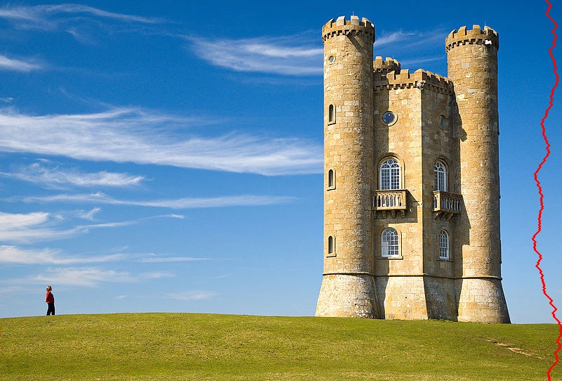
In the image above, you can see the seam² with the least energy that will get removed.

Finally, you can repeat all of these steps if you want to shrink an image more than just one pixel. In the video below you can see all the seams that are chosen to get the original image to half its width without distorting the image.

Remarks #

Of course, it’s perfectly possible to resize an image in the height as well. The same concept and techniques apply and both dimensions can be resized at the same time too.

Performance-wise you can also make some optimisations. Think of splitting some work to do in parallel (using the Web Workers API) or not doing some operations over and over again (e.g. turning the shrunk image greyscale again).

Demo and resources used #

The code is located at my GitHub repository and a demo can be found here.

Wikipedia - Kernel (image processing)
Wikipedia - Sobel operator
Wikipedia - Convolution
Wikipedia - Seam carving